
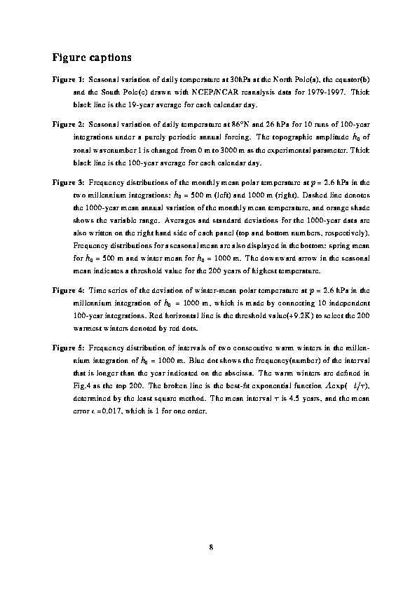
Figure 1: Seasonal variation of daily temperature at 30hPa at the
North Pole(a), the equator(b) and the South Pole(c) drawn with
NCEP/NCAR reanalysis data for 1979-1997. Thick black line is the
19-year average for each calendar day.
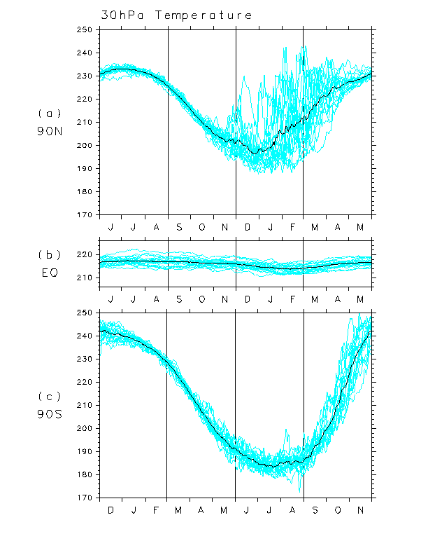
Figure 2: Seasonal variation of daily temperature at 86N and 26 hPa
for 10 runs of 100-year integrations under a purely periodic annual
forcing. The topographic amplitude h_0 of zonal wavenumber 1 is
changed from 0 m to 3000 m as the experimental parameter. Thick black
line is the 100-year average for each calendar day.
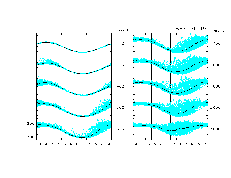
Figure 3: Frequency distributions of the monthly mean polar
temperature at p = 2.6 hPa in the two millennium integrations:
h_0 = 500 m (left) and 1000 m (right). Dashed line denotes the
1000-year mean annual variation of the monthly mean temperature, and
orange shade shows the variable range. Averages and standard
deviations for the 1000-year data are also written on the right hand
side of each panel (top and bottom numbers, respectively). Frequency
distributions for a seasonal mean are also displayed in the bottom:
spring mean for h_0 = 500 m and winter mean for h_0 =
1000 m. The downward arrow in the seasonal mean indicates a threshold
value for the 200 years of highest temperature.
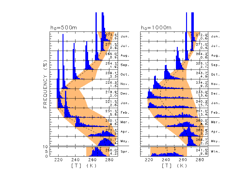
Figure 4: Time series of the deviation of winter-mean polar temperature
at p = 2.6 hPa in the millennium integration of h_0
= 1000 m, which is made by connecting 10 independent 100-year
integrations. Red horizontal line is the threshold value(+ 9.2 K)
to select the 200 warmest winters denoted by red dots.
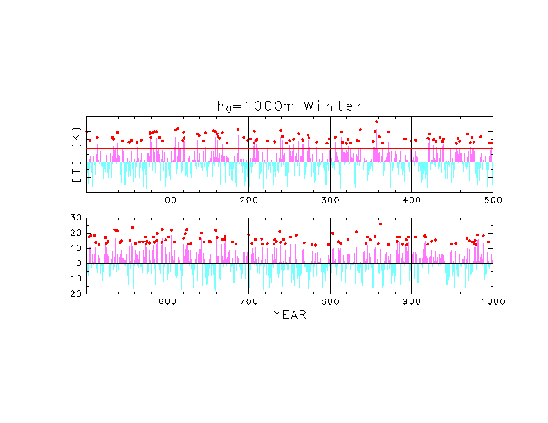
Figure 5: Frequency distribution of intervals of two
consecutive warm winters in the millennium integration of h_0 =
1000 m. Blue dot shows the frequency(number) of the interval that
is longer than the year indicated on the abscissa. The warm winters
are defined in Fig.4 as the top 200. The broken line is the
best-fit exponential function A exp(-t/T), determined by the
least square method. The mean interval T is 4.5 years, and
the mean error epsilon = 0.017, which is 1 for one order.
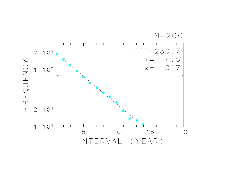
Figure X1: 対流圏─成層圏結合系の季節内変動。極域温度偏差(上)、中緯
度帯状平均東西風(中)、ジオポテンシャル高度場の帯状波数1成分の振幅
(下)の高度─時間断面図。
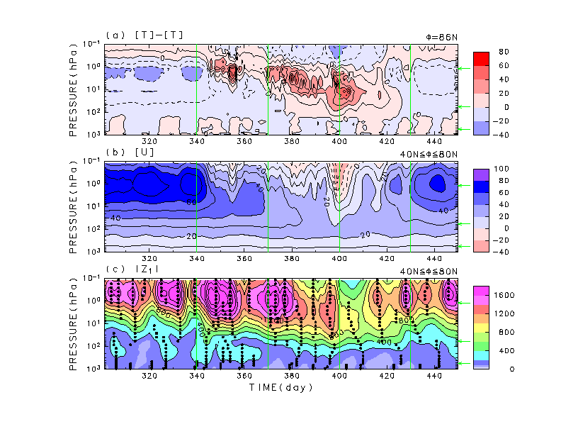
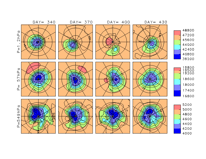
Figure X2: 周極渦の時間変動。30日毎のジオポテンシャル高度場。上部成
層圏(上)、下部成層圏(中)、対流圏(下)。
